VERIQA and the Mysterious CHAIR
On Sept 4th 2024, two months after commissioning, the VERIQA calculation counter showed 1043. This means that more than 10 plans per day were MC calculated during the first two months1, and the success story could end here.
The remarkable agreement between RT MonteCarlo 3D dose and Eclipse (especially Acuros) dose, which is the basis for a successful and worry-free routine application of the VERIQA workflow, was achieved through fine-tuning of our beam models. During testing, we had noticed a dose discrepancy for small moving slits (the "Gap"-fields). We had compensated this by adding a small Leaf Offset Correction (LOC) to each beam model. The best dose agreement for the "Gap4" target plan (4 mm wide slit) was found with LOC values between 0.08 and 0.11 mm, depending on energy.
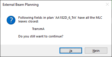
However, a small dose discrepancy was left which we could not compensate: It concerned static leaf transmission. Hardly worth mentioning, because it only showed up for nonclinical fields fully blocked by the MLC2, it was still there. Although being totally happy with VERIQA's overall clinical performance, we still felt that this deserves a follow-up.
An Experimental Beam Model
When the SciMoCa™ beam models are generated by PTW for a treatment machine like a TrueBeam equipped with, say, HD120 MLC, the geometrical and physical parameters of the MLC (e.g., leaf dimensions and material of thick and thin leaves) define the radiation physics, and the transmitted dose is an output. When the Eclipse user sets up his calculation models however, the transmission factor (e.g., 1% for 6X) is an input.
There is no such thing as "transmission factor" during linac head modelling. Fortunately, a so called Leaf Gap (LG), which describes the width of the air gap between adjacent leaves (neighboring leaves on the same leaf bank), can be used to tweak the MC beam model.
We reached out to PTW and asked them to optimize an experimental 6X beam model for leaf transmission. The goal was to improve agreement for the transmission plan already mentioned.
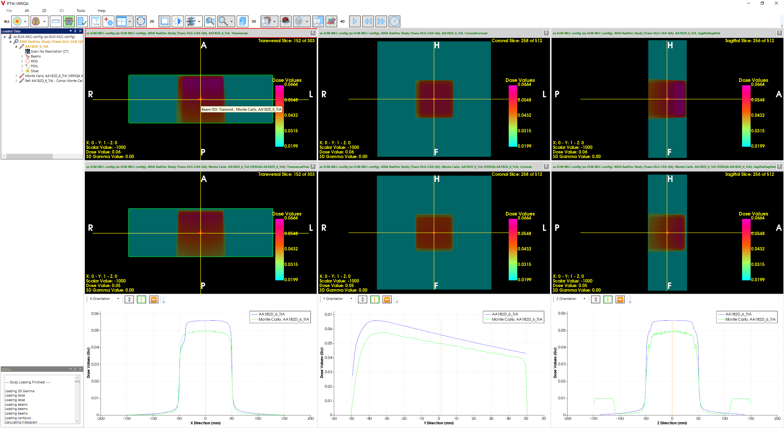
A few days later, we received the test model from PTW. We learned that while our commissioned 6X model uses an LG of 0.09 mm, they found better agreement for the transmission plan after increasing the LG to 0.12 mm, which is a minimal change of only 30 µm:
(Dose through MLC-blocked field using 6X test model optimized for leaf transmission by PTW.)
To be able to test the experimental beam model with other Eclipse plans, we first had to solve a problem: the commissioned "production" models cannot be used in parallel with experimental models. When a 6X plan for TrueBeam_BLAU or TrueBeam_GRUEN is sent from Eclipse to VERIQA, VERIQA cannot decide whether to use the experimental or the commissioned beam model.
One solution would be to set up a third linac (e.g., TrueBeam_GELB, 6X only) in the ARIA database in addition to the two existing machines. Plans generated for TrueBeam_GELB in Eclipse would be routed automatically to the experimental beam model in VERIQA. However, setting up a third TrueBeam in ARIA only for testing purposes seemed too invasive to us, because treatment machines cannot be deleted anymore.
A simple, less invasive alternative is to export the plan as a file, edit it with an editor, and forward the edited plan to VERIQA.
In Eclipse, in addition to the existing VERIQA DICOM Storage Export Filter we set up a DICOM Media File Export Filter, which saves plan files to an intermediate folder. There, we open the RP-File (the Plan file) and edit the Treatment Machine Name in DICOM tag (300a,00b2) using DicomEdit™ 1.7 from Varian:
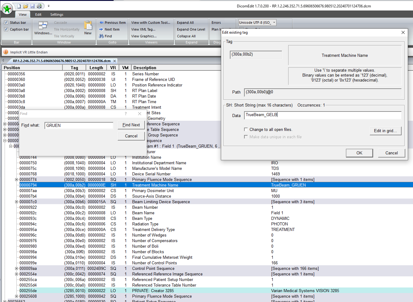
(DicomEdit™ is used to change the Treatment Machine Name.)
In the example, we replaced TrueBeam_GRUEN by TrueBeam_GELB in a single DICOM tag3.
The final step is to send the modified dataset (RS-, RD- and CT-files remain unchanged) from the intermediate folder to VERIQA for calculation. We do this with RT View. We open the dataset using "Load Local Dataset", and then select "Save Active Dataset", specifying the veriqascp host as the DICOM destination. This sends the dataset with the edited plan to VERIQA. The plan is automatically calculated, because VERIQA finds a matching radiation unit (TrueBeam_GELB) with a 6X beam model. This way, any 6X plan can be calculated using the experimental model.
Checking Leaf Offset Correction
With the commissioned models, we had used a small Leaf Offset Correction in order to get gap dose right. What LOC should be used with the experimental model?
When PTW sends new beam models to the customer, the LOC is never part of the package. It simply does not exist at this stage. Only in the local VERIQA installation, after the beam models are imported and tested, the user may define a leaf offset correction if it seems necessary.
A nonzero, positive LOC will add a small distance to all leaf positions. Gaps between opposing leaves will become wider, increasing dose. The "Leaf Gap" PTW was modifying for the experimental model is a different thing: it acts perpendicularly to the LOC if you will, because increasing the LC increases the air gap between neighboring leaves, a zone of higher leakage (which MLC manufacturers try to minimize by using the tongue-and-groove design).
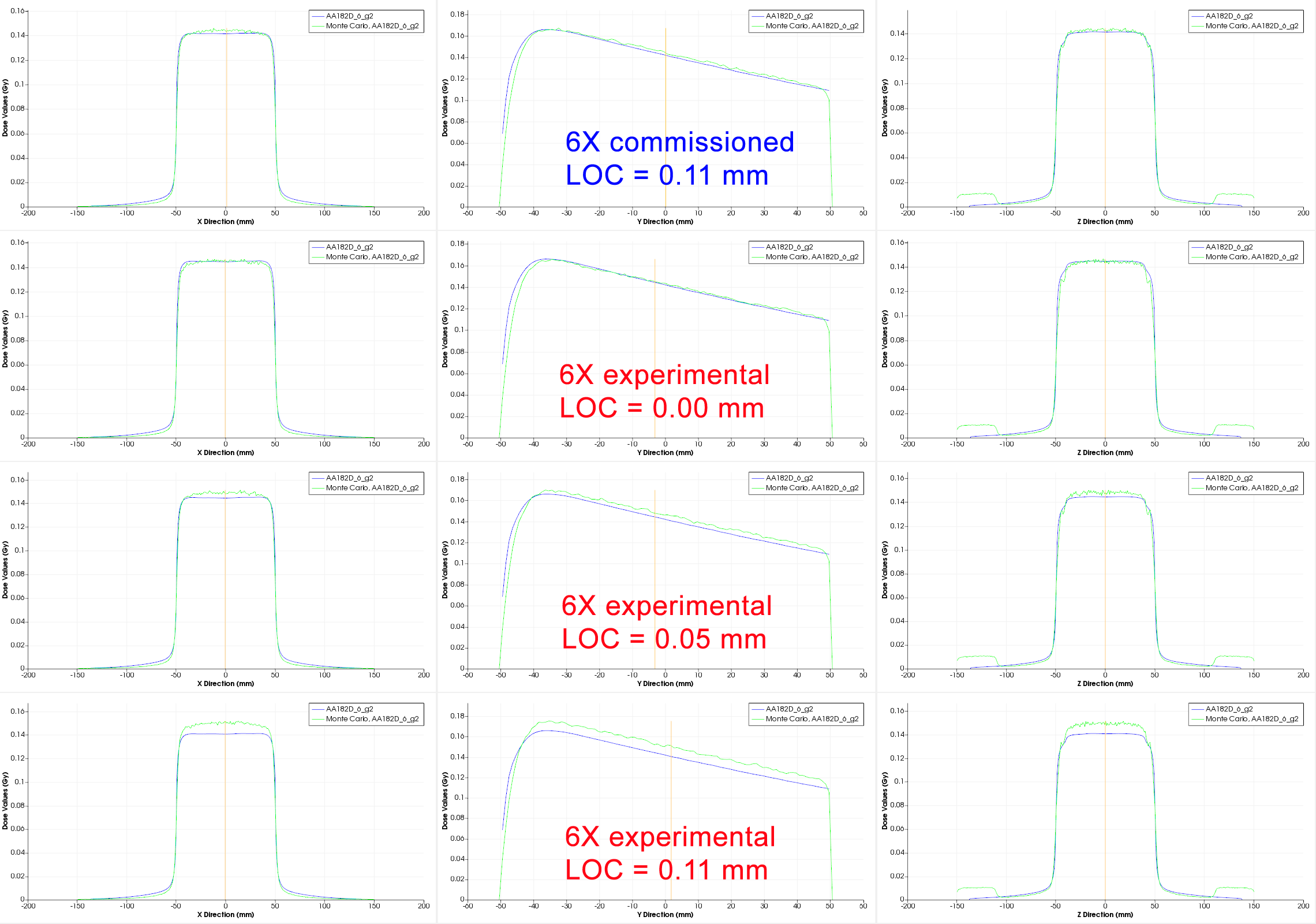
To make sure that we understand this correctly, we calculated several test plans with three different LOC settings (0.00 mm, 0.05 mm and 0.11 mm) in the experimental model. As long as a beam model is not commissioned in VERIQA, it is easy to change the LOC and recalculate a plan. Evaluations, as usual, are performed as dose profile comparisons in RT View.
The Gap4 field is the primary test plan for our dose check. It is an interesting result that for the experimental beam model, the version without any leaf offset correction (LOC = 0.00 mm, second row) gives the best fit:
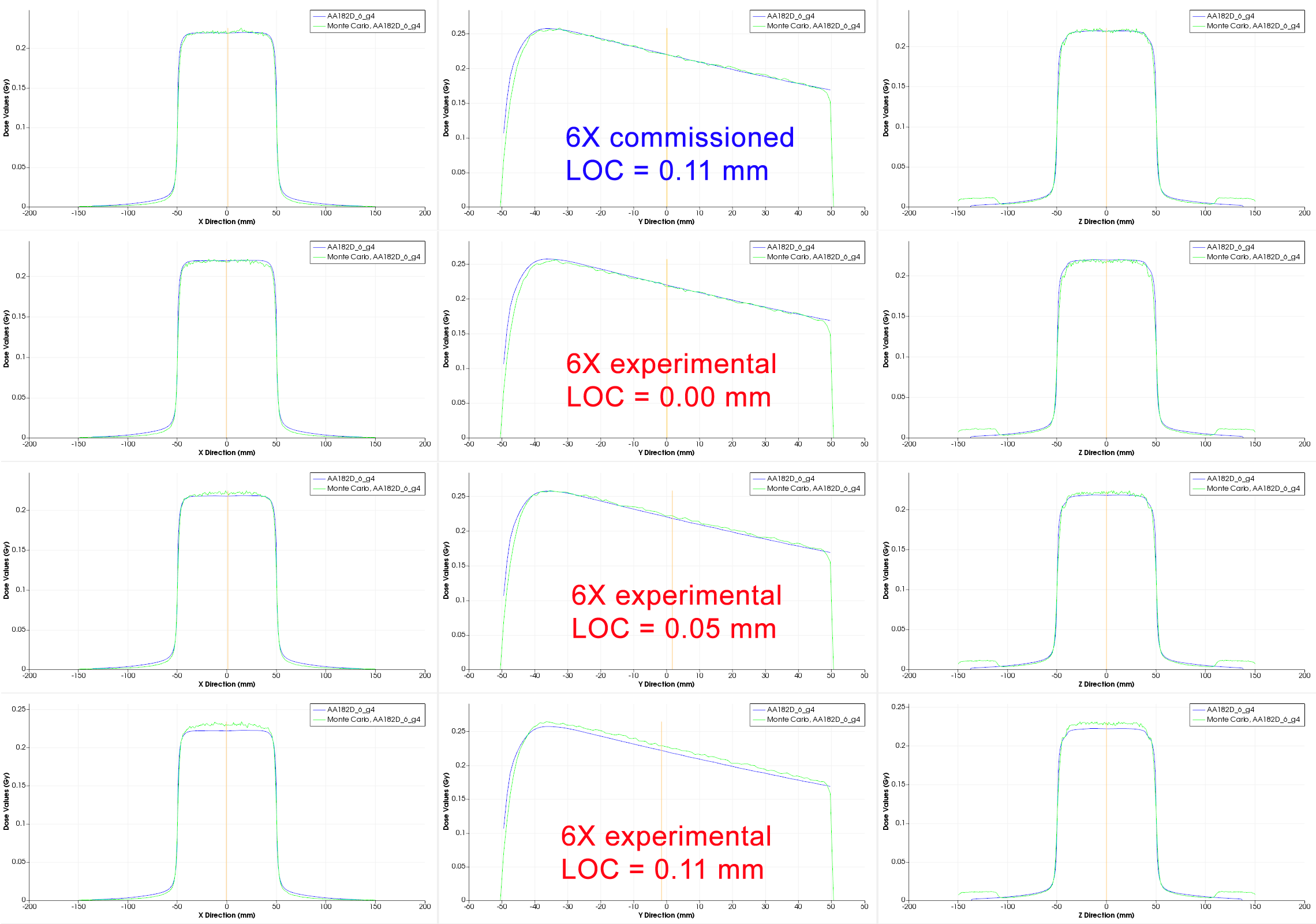
(The Gap4 field in RT View dose profile comparison. Left: crossplane profile in 5 cm depth in direction of leaf movement, center: PDD, right: inplane profile)
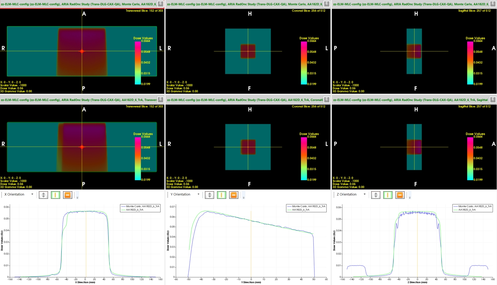
The same holds for the even narrower 2 mm gap (Gap2 field). Generally speaking, the smaller the moving gap, the larger the influence of adding a fixed offset:
(The Gap2 field in RT View dose profile comparison. Click to enlarge.)
It may be a coincidence in our experimental model, but it looks like the improvement in the model for the static leaf transmission renders the LOC obsolete: as we have seen, the Leaf Offset Correction can remain at the default value of 0.00 mm.
The Mysterious CHAIR
Now that we have checked gap dose for our experimental model in the same way as we did for the commissioned models, we want to come to the clickbait part of the title, the "Mysterious CHAIR".
For more than 20 years, this simple dynamic test pattern has been giving us headaches, because it never worked well in dose verifications, no matter whether the measurements were performed with a 2D Array or with Portal Dosimetry. There was often a "problem" in the upper part of the pattern.
Depending on the exact implementation of the CHAIR (size, MU, gap width, depth of comparison), dose agreement could be better or worse. For "pain relief", a larger target dose can be chosen, which leads to wider gaps when the Leaf Motion Calculator4 is asked to generate a DMLC field (e.g., by selecting F11 in Eclipse). If gaps are wide, dose agreement is typically better. But if the moving slit in the upper part (the "back" of the CHAIR) is narrow enough, deviations between Eclipse and measurement can become quite large. In order not to confuse results, we want to focus on a certain fixed implementation of the CHAIR:
(This is the CHAIR we are talking about. 61MU@600MU/min result in a gap width in the upper part of about 4 mm.)
During VERIQA commisioning, we checked several test patterns, and the CHAIR of course was on the list5. How did it perform? Besides the comment on a small mismatch regarding static transmission (which triggered this story), it was excellent. There is not much to complain about this inplane profile:
Now where is the pain?
So far, the only two advantages of our experimental model over the commissioned model are that:
- transmission dose is better, and
- no LOC is needed.
However, this is not enough motivation for us to ask PTW to repeat the procedure for the other four energies as well. We would have to repeat the commissioning process for all five energies, decommission the now commissioned models (remember: excellent agreement!), and commission the transmission-improved models instead.
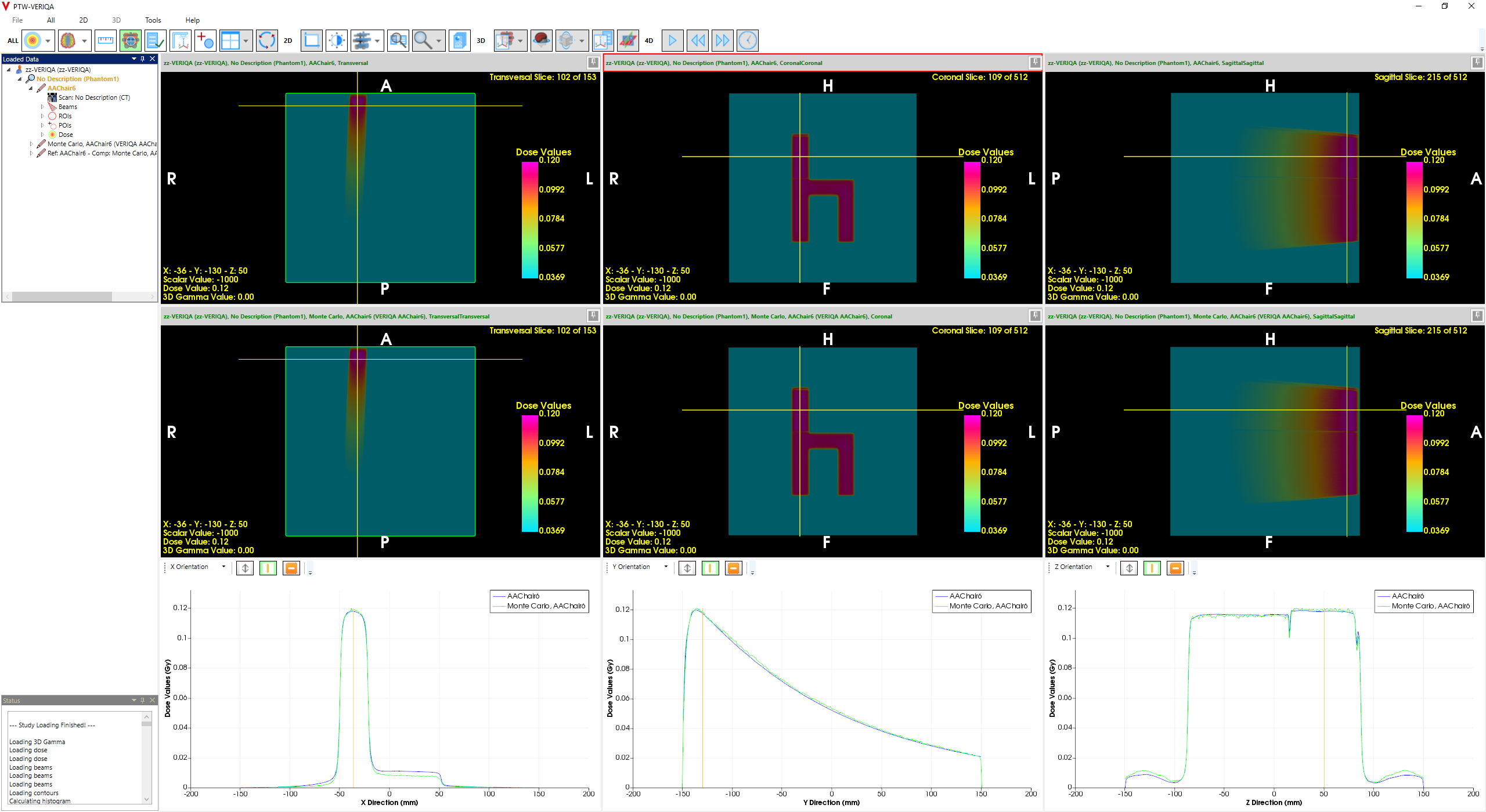
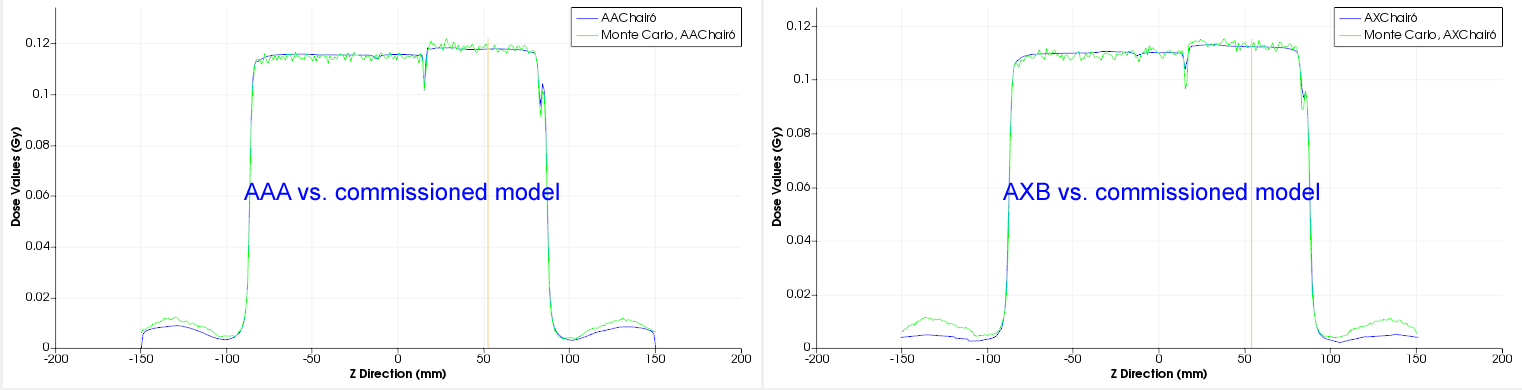
How does the experimental model calculate the CHAIR?
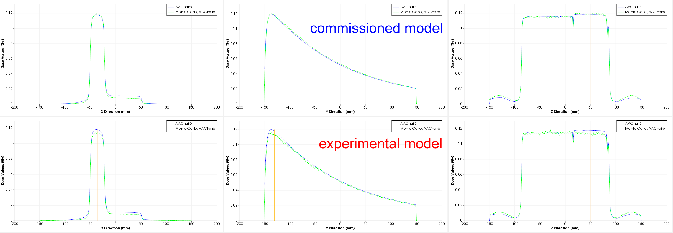
(The two MC models in comparison with AAA calculation of the CHAIR. Click to enlarge.)
In the upper part of the CHAIR, AAA agrees better with the commissioned model (blue arrow) than with the experimental model (red arrow). We cannot say that this increases our motivation to switch models. Rather the contrary.
But what if Eclipse in this specific case is "wrong" and the experimental MC model is "right"? We already noted in the Discussion: "One should be aware that in the described process, we tried to minimize the dose discrepancy between TPS and MC, while ideally, the MC model should be compared to measurements, not TPS dose." Our assumption "TPS dose is interchangeable with measured dose" is only an assumption, which is justified by the fact that the TPS is thoroughly tested. But is this assumption valid for all possible cases?
The easiest and fastest way to get a reliable measurement result for the "mysterious CHAIR" is to use portal dosimetry together with EPIQA (version 5.4.005). Measurement depth here is dmax:
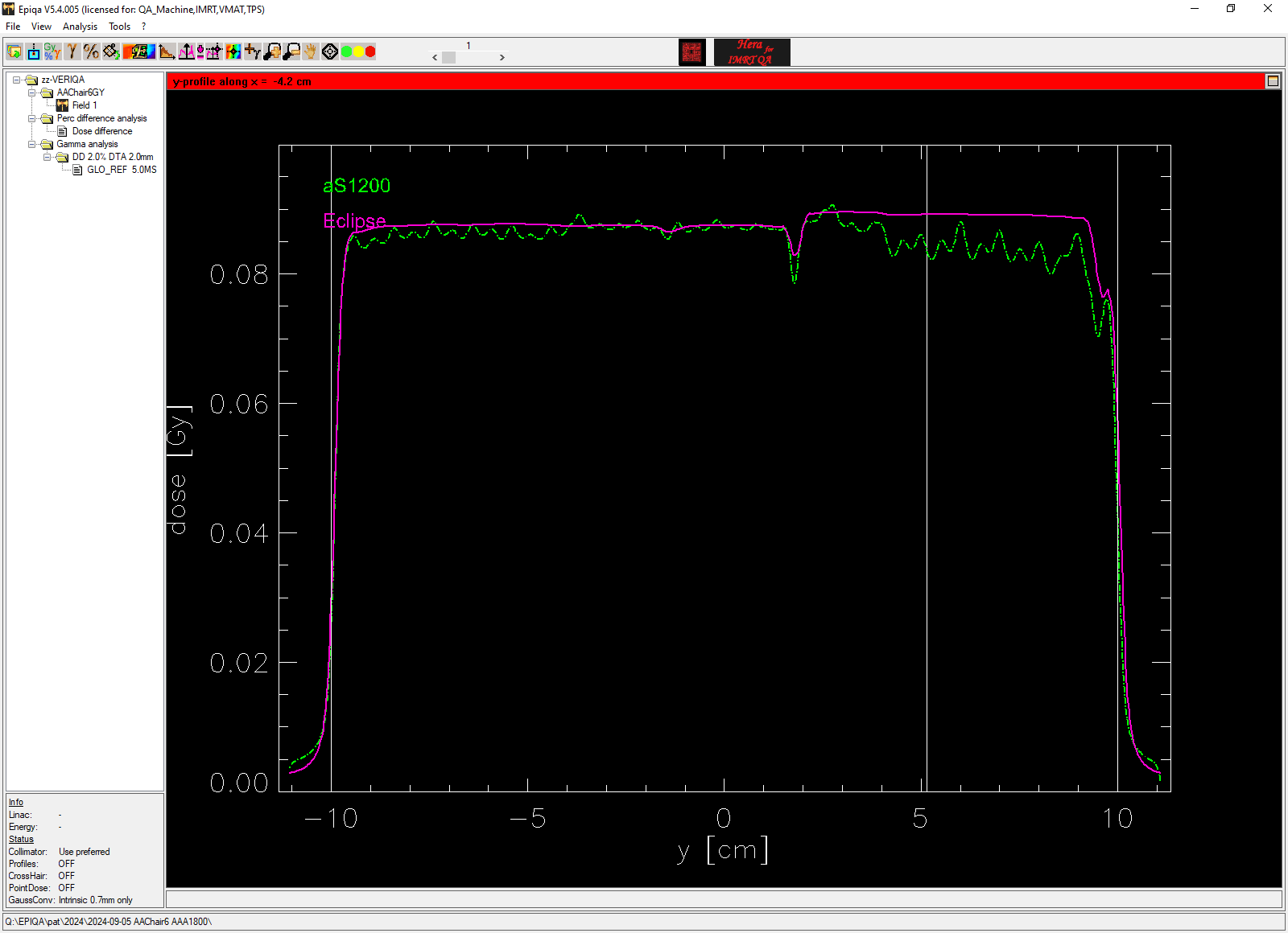
EPIQA evaluation: AAA dose (left) vs. portal dose (right). 2%/2mm Gamma map (center).
Now this is an interesting result. In the upper part of the CHAIR, the green EPIQA profile (arrow) drops in the same way as the experimental MC model, while the Eclipse profile (magenta) remains flat.
Until now, when thinking about the possible reasons of the dose discrepancy, we had often suspected a shortcoming in the measurements, especially with a 2D Array. The next image shows a comparison of the AAA-calculated CHAIR (upper left) and a measurement with the PTW OCTAVIUS Detector 1500 (lower left). MU were scaled by 5 without changing leaf motions. Measurement depth is 5 cm. The PTW VeriSoft evaluation confirms the EPIQA result regarding the profile (arrow):
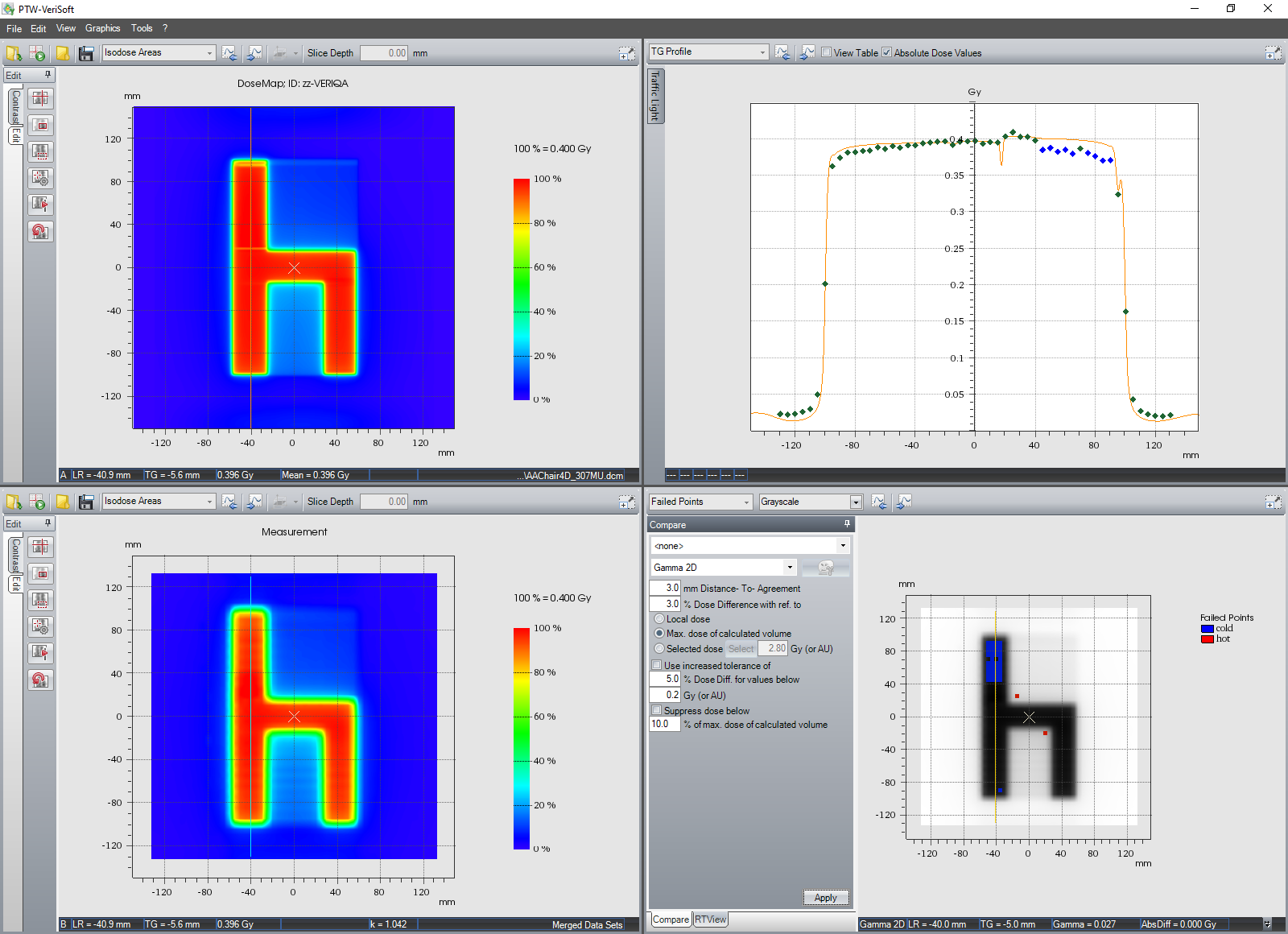
(VeriSoft evaluation of the CHAIR measured with the OCTAVIUS Detector 1500.)
Thanks to VERIQA, our perspective has changed in that we now also consider that the cause of the deviation could lie in the planning system.
What does this mean for the Eclipse algorithms? Why is the calculated profile too high?
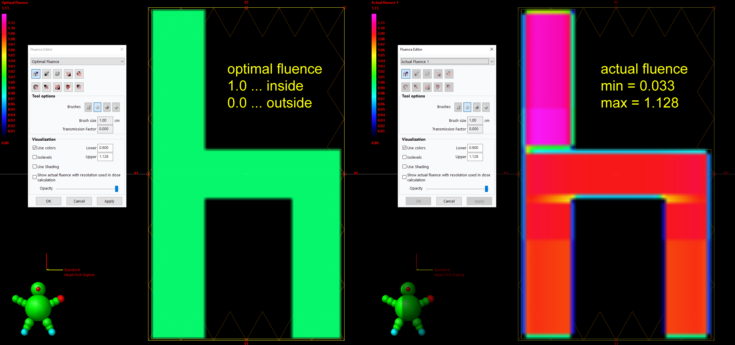
The source of the CHAIR is an optimal fluence pattern which can be imported or painted "by hand" in Eclipse6. The intensity value of optimal fluence set to 1.0 in most areas of the CHAIR, and zero elsewhere (see next image). This optimal fluence pattern is then converted to the actual fluence by the Leaf Motion Calculator (SmartLMC in our case), and finally to dose by the dose calculation algorithm (AAA or AXB).
In the inplane dose profiles of the EPIQA evaluation, the part of the Eclipse profile which is to the right of the tongue-and-groove "dip" is at a higher level than the part left of the dip. This is not plausible, since the optimal fluence in this region is not higher than in other parts of the CHAIR.
In Eclipse, not only the optimal fluence can be visualized (which is needed for "fluence painting" in the first place), but also the actual fluence. It can clearly seen that the actual fluence shows the higher intensity in the upper part of the pattern:
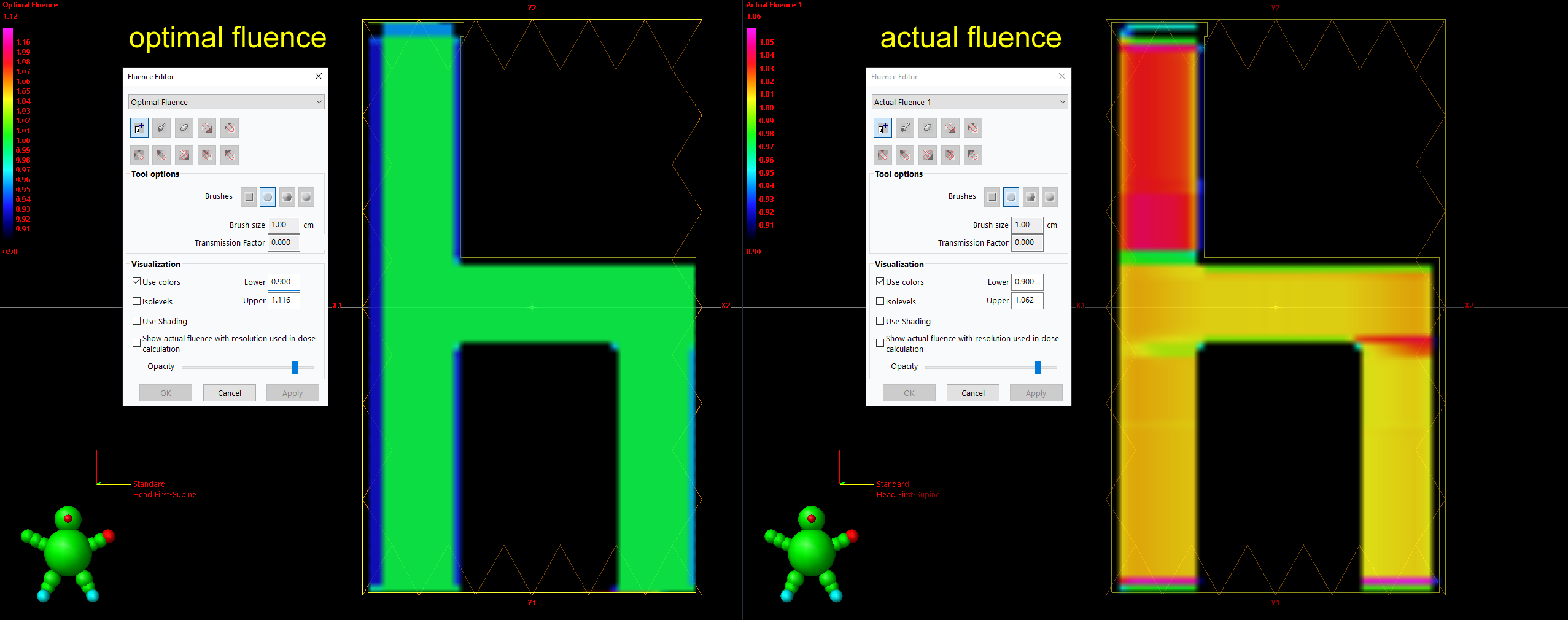
(Eclipse: optimal and actual fluence of the CHAIR7.)
If the actual fluence is higher, dose will be higher, too.
Interestingly, there is a second leaf motion calculator which is older and which does not show the described behaviour of the Smart LMC: the Varian Leaf Motion Calculator (LMCV) is still available in Eclipse version 18. It is less sophisticated and has other shortcomings (no support for Jaw Tracking, no fractional MU, etc.), which is why SmartLMC clearly is the better choice for clinical IMRT planning. But why SmartLMC behaves that way for the CHAIR and the specific set of input parameters - we don't know.
For now, we can only conclude that the "Mysterious CHAIR" deserves its name.
Notes
1 The counter showed 595 at the time of commissioning, which means that in 43 working days, 448 plans were calculated.
2 Eclipse even gives a warning before calculating.
3 If an AXB plan is calculated using Plan Dose Calculation (our default), the Treatment Machine Name only appears once in the DICOM plan file. If Field Dose Calculation is used instead, the number of occurrences depends on the number of fields.
4 We always select Jaw Tracking = OFF for test fields such as the CHAIR.
5 We put it in the section "Complex IMRT Fields", although it is actually rather simple.
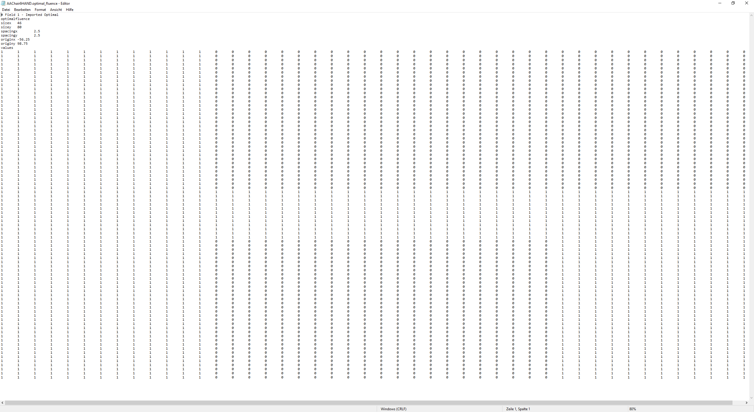
6 The imported optimal fluence was generated out of a greyscale TIF image which was converted to an Optimal Fluence file (*.txt format) via home-made MATLAB script. In clinical IMRT planning, the 2D distribution of optimal fluence is the result of an inverse optimization process.
7 Only if the optimal fluence is painted by hand instead of converting a TIF image, perfect results can be achieved, i.e., the optimal fluence matrix consists only of zeros and ones.