
In July 2012, we installed three new Eclipse modules: Conformal Optimization (CO) , Biological Optimization and Biological Evaluation, all developed by RaySearch Inc.. The versions that come with Eclipse 13.0.33 are now mature enough so that they can be used clinically (see sidebar on previous versions):
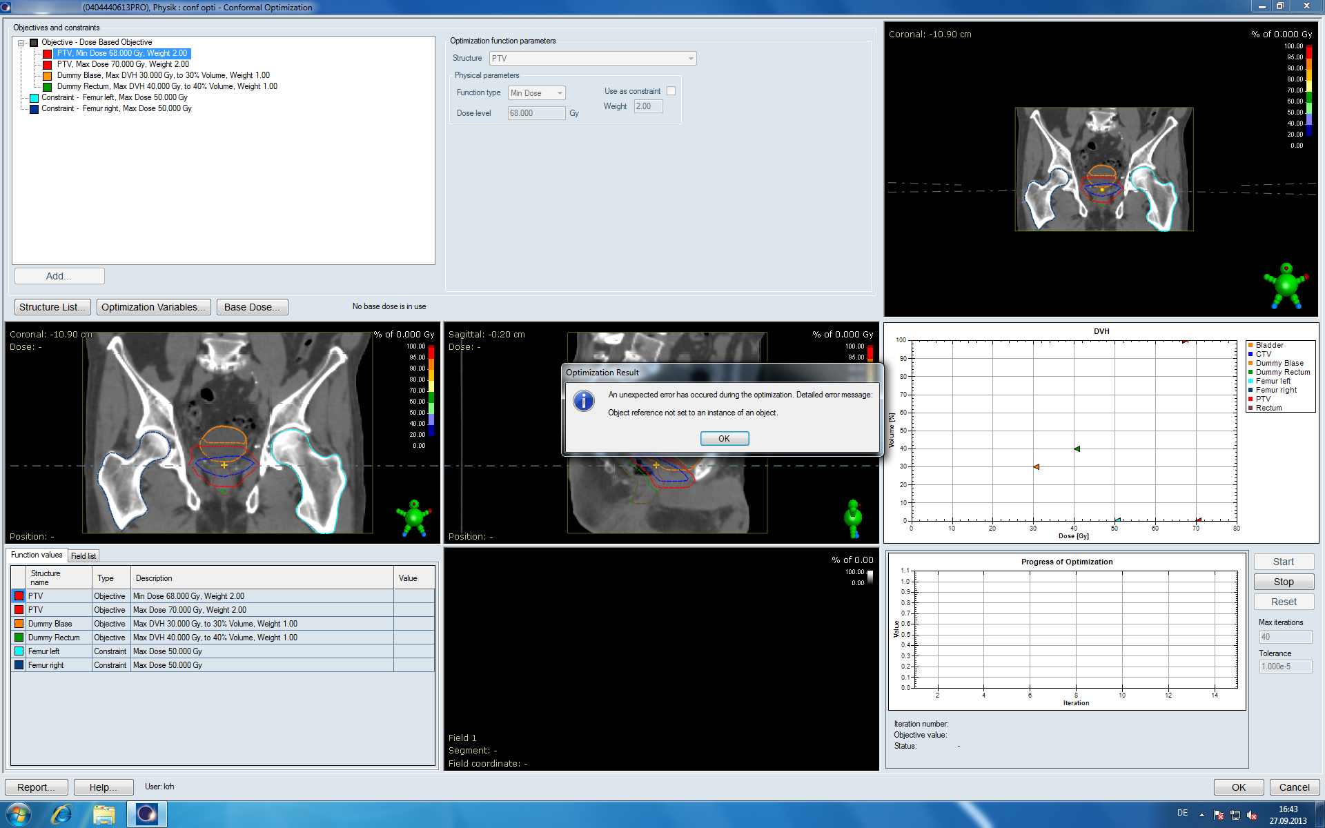
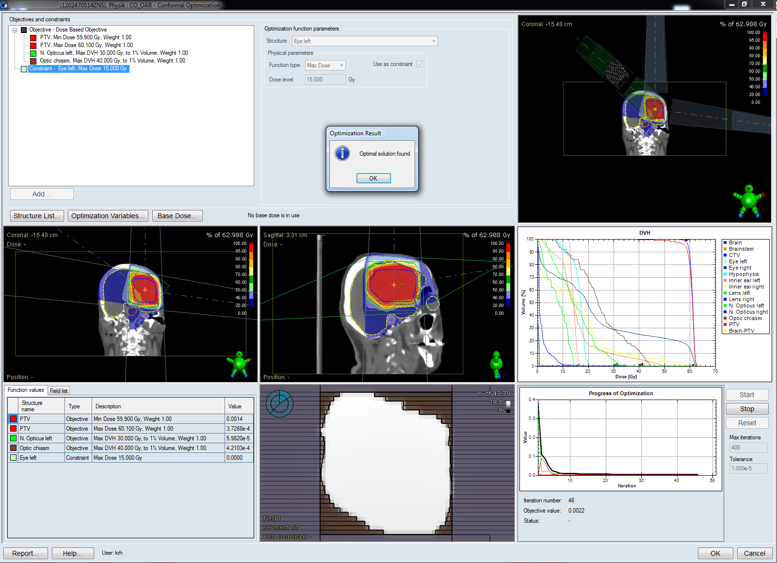
(User interface of Conformal Optimization.)
The Idea Behind Conformal Optimization
A conformal treatment plan typically contains several static fields (dynamic wedges however are perfectly fine). Target conformation is achieved via static MLC shapes. In a forward-planned conformal plan, the machine parameters such as gantry angle, collimator angle, couch angle, wedge angle, as well as the leaf shapes are set by the user based on his/her experience. After 3D dose has been calculated, field weights are sometimes adjusted manually to improve plan quality.
It is not hard to imagine that the "solution" found by the user will probably not be the optimal one (considering the millions of possible combinations of the aforementioned machine parameters alone). This is where CO comes into play. In an optimization loop, CO tries to minimize an objective function by varying user-selected parameters such as gantry or wedge angle. The whole optimization process is really very similar to IMRT, with the exception that in-field fluence can only be "modulated"1 to some extent with the help of wedges, but not with a dynamic MLC.
Preparing a Plan
Before CO can be launched, a static plan with the desired number of fields, static MLC, and proper isocenter has to be set up. CO will not change isocenter during optimization (it could, however, reduce the field weight of a certain field to zero if it finds that the field is unnecessary).
In the following example, a glioblastoma patient shall be optimized. We create a three field plan with initial settings of gantry angle. One of the fields is non-coplanar.
A valid treatment prescription (30 times 2 Gy to the target volume PTV) must also exist.
Interfacing with Eclipse
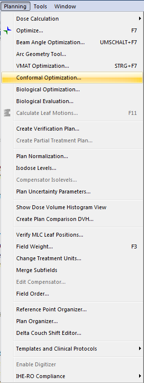
In Eclipse 13, CO is launched by selecting Conformal Optimization in External Beam Planning's Planning menu. The workstation then switches to the RaySearch user interface2, which takes about 15 seconds.
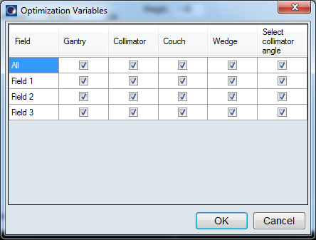
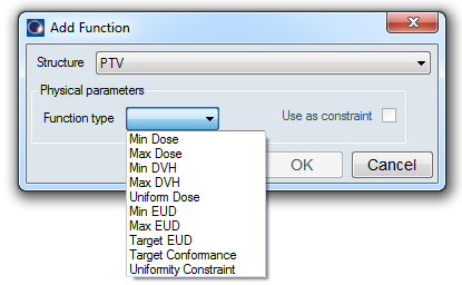
Via the Add ... button, we define two objectives for the PTV, a Min Dose and a Max Dose objective (one could as well use DVH Objectives). We select all of the possible Optimization Variables: gantry, collimator, couch and wedge angle shall be optimized. Select collimator angle means that CO will perform an initial collimator rotation to match the shape of the target3.
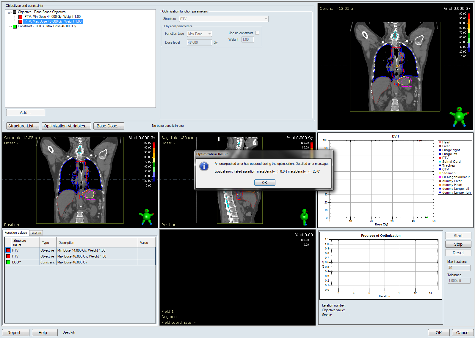
We hit the Start button and watch the graphics:
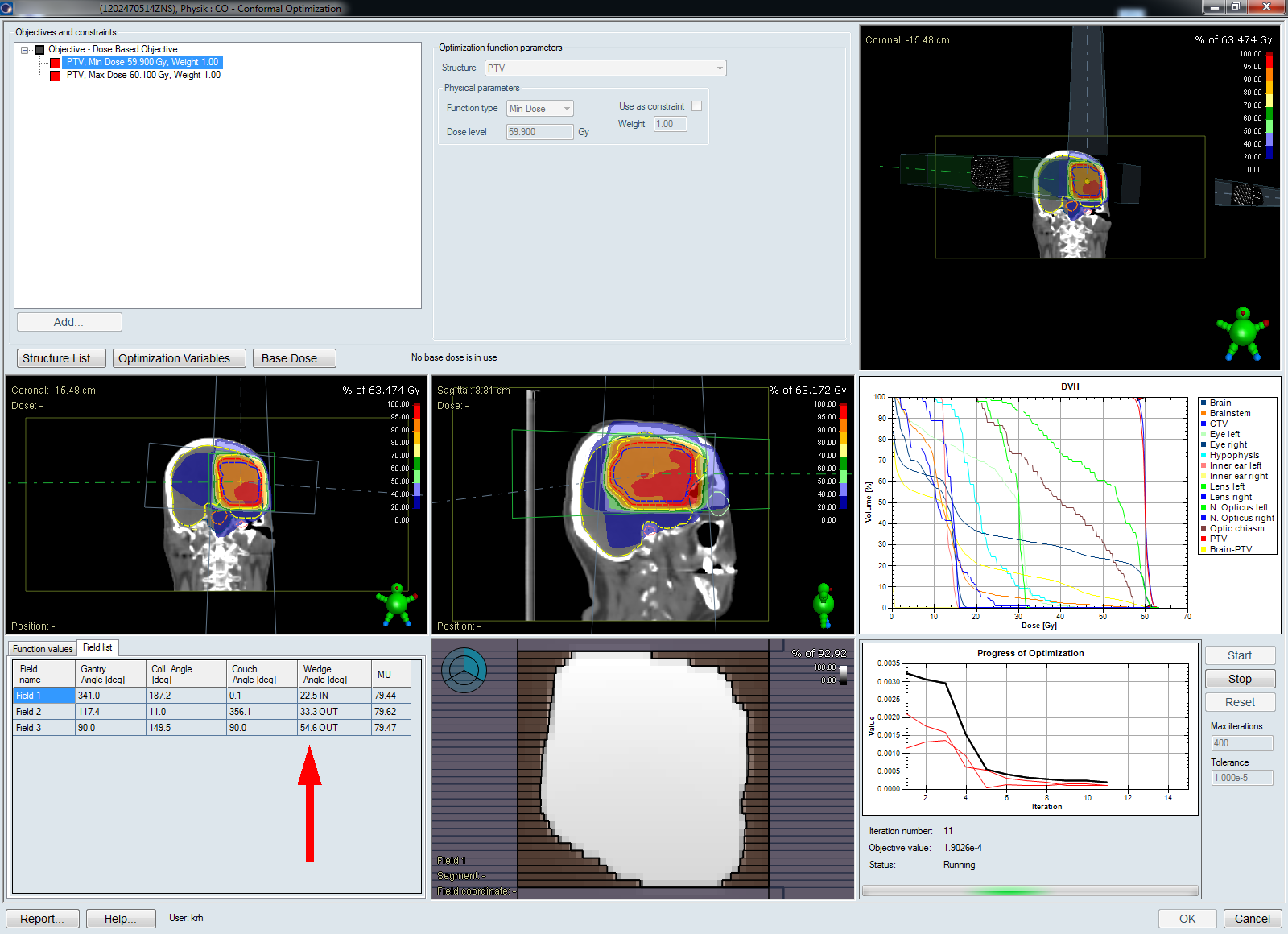
All sub-images of the user interface can be expanded to fullscreen. Patient views can be rotated as well. The tab named Field list in the lower left corner displays the current wedge angle (red arrow). During optimization, the angle can be a continuous value and does not necessarily match the angles available on the treatment machine (10°, 15°, ... , 60°):
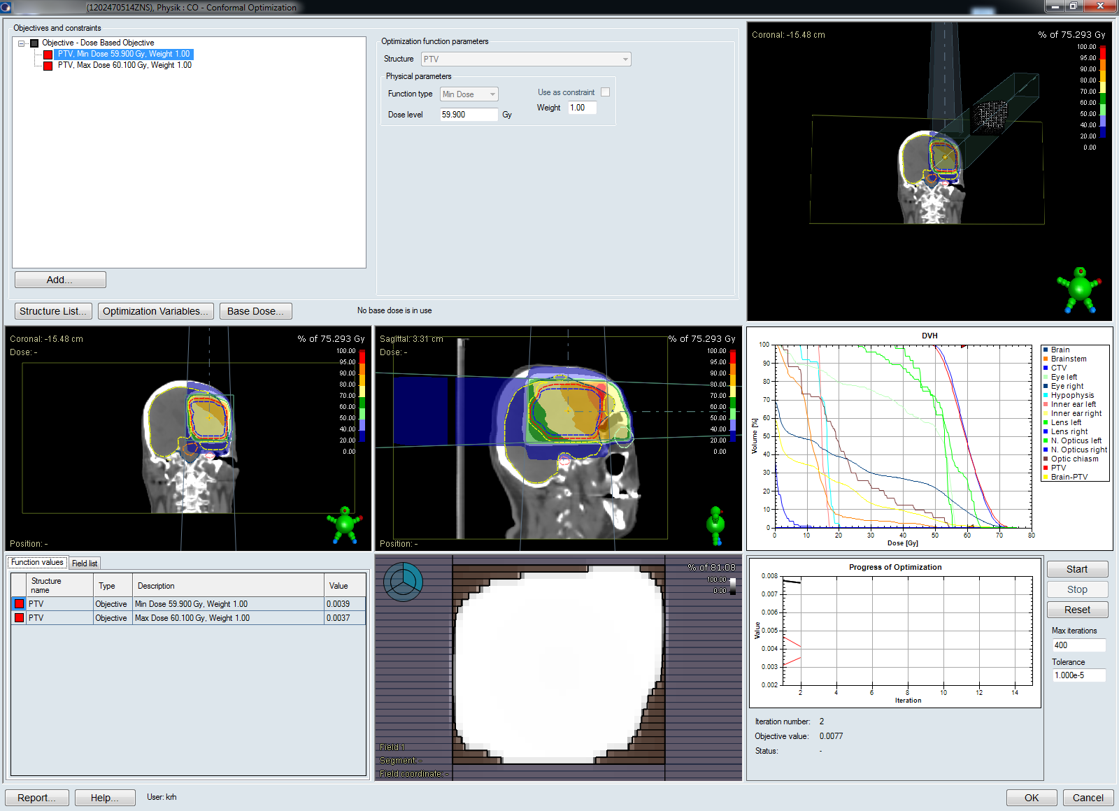
When CO stops, all values are rounded to deliverable values. This can trigger a small final increase of the objective value:
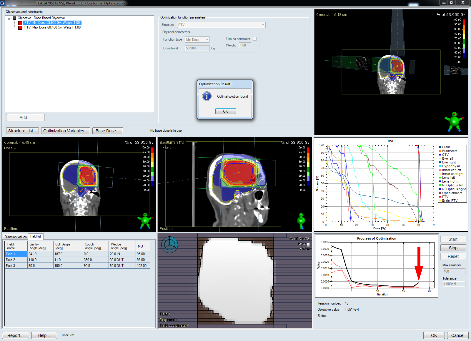
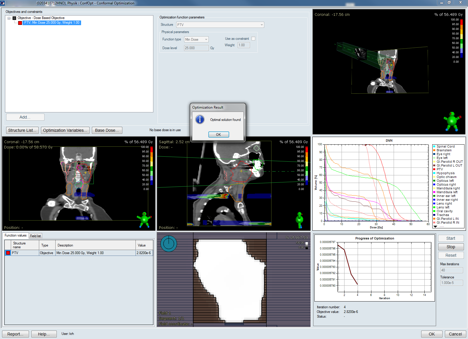
CO will either stop after Max iterations or when the change in the objective value indicates that an optimal solution has been found.
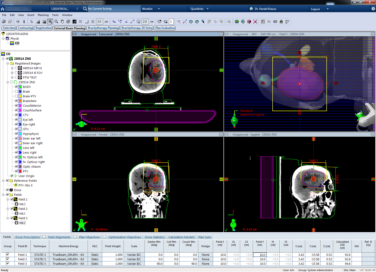
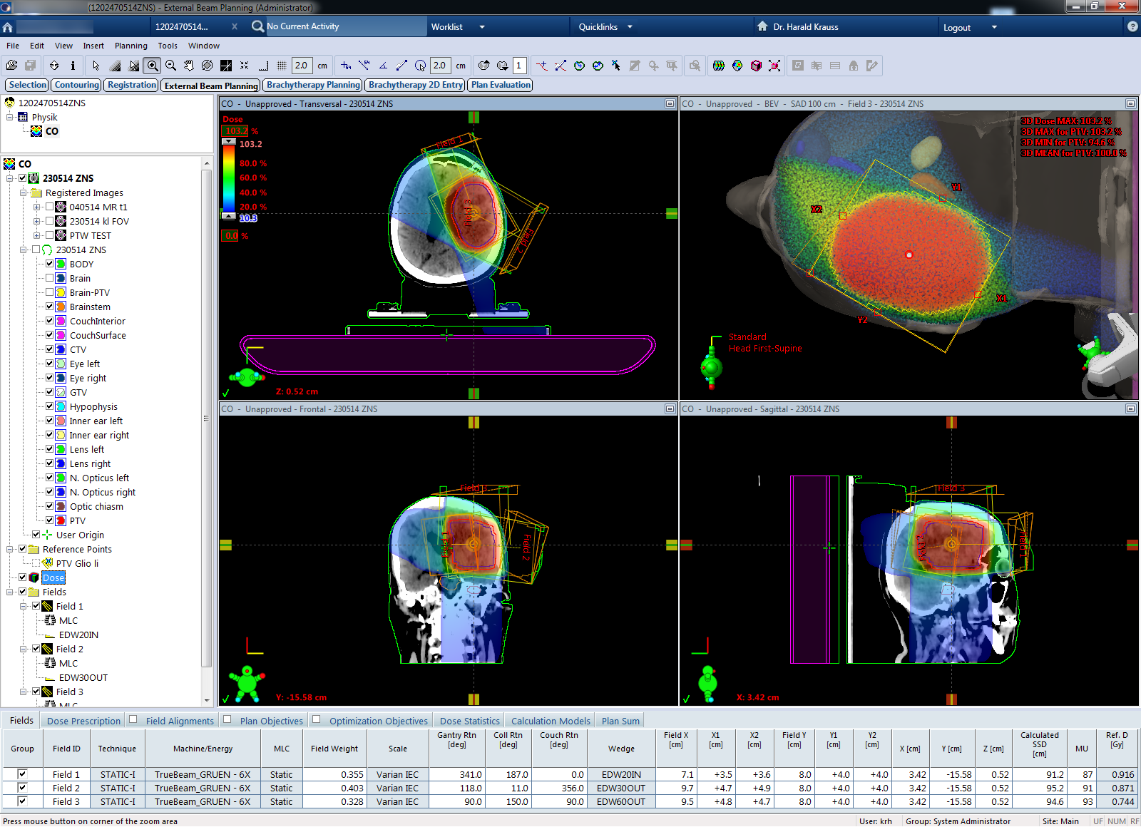
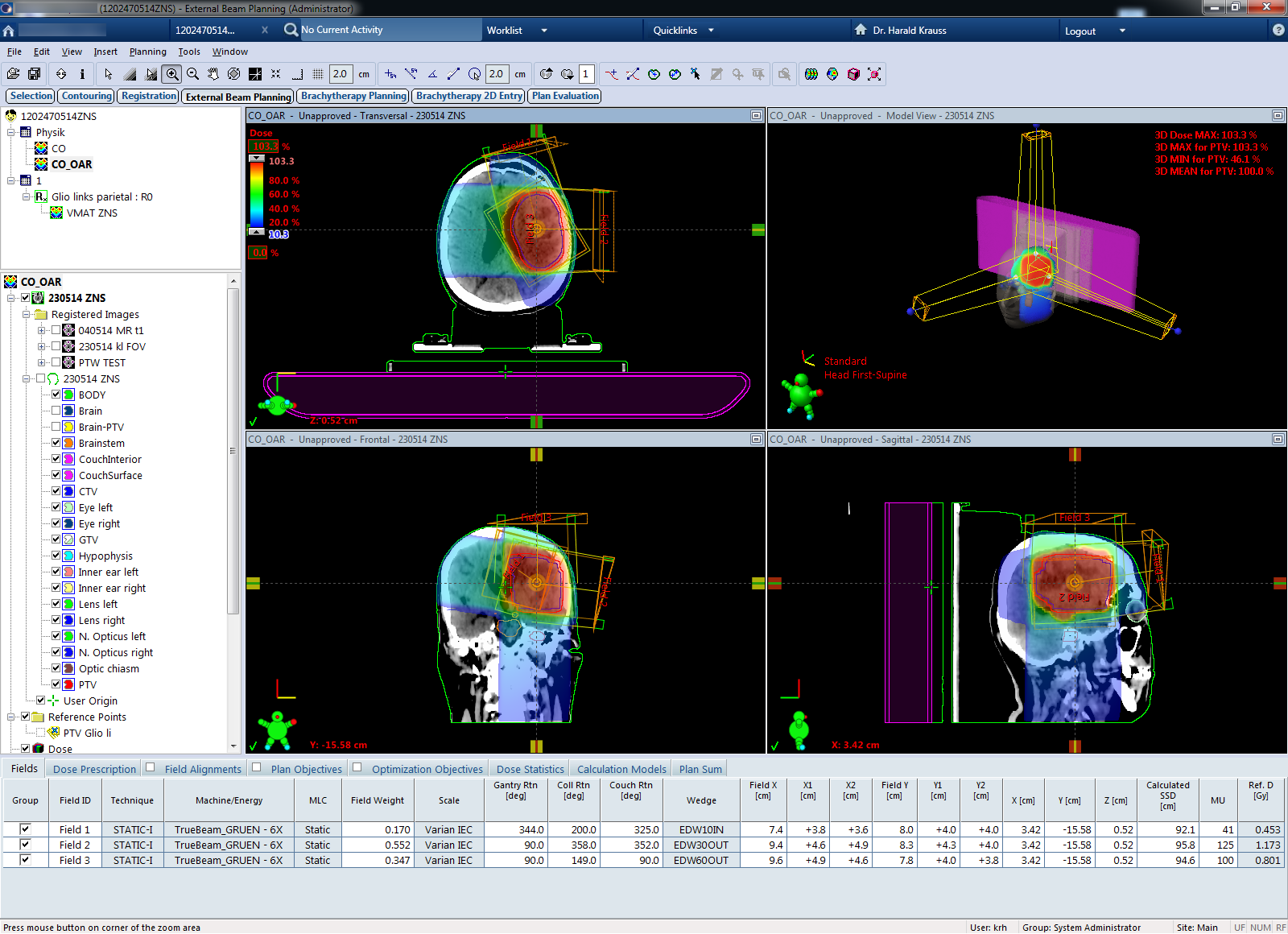
After clicking OK, Eclipse switches back to External Beam planning, and 3D dose can be calculated with AAA:
How Good Does it Work?
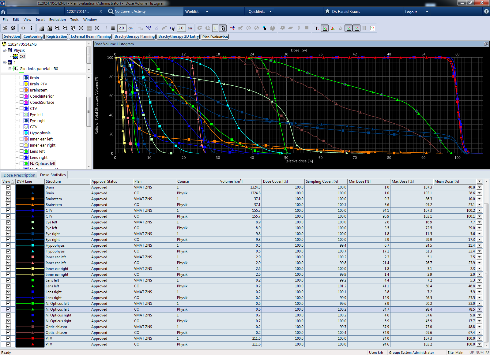
The above example plan was optimized for the target structure PTV alone. As a consequence, a comparison with the clinical VMAT plan is not fair: regarding dose conformality (PTV Min 94.6%, PTV Max 103.2%), the CO plan is better than the VMAT plan (PTV Min 84.0%, PTV Max 107.3%). But this is only part of the story. Some OARs in the CO plan (triangles in the plan comparison) would receive too much dose:
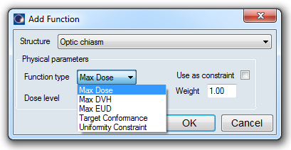
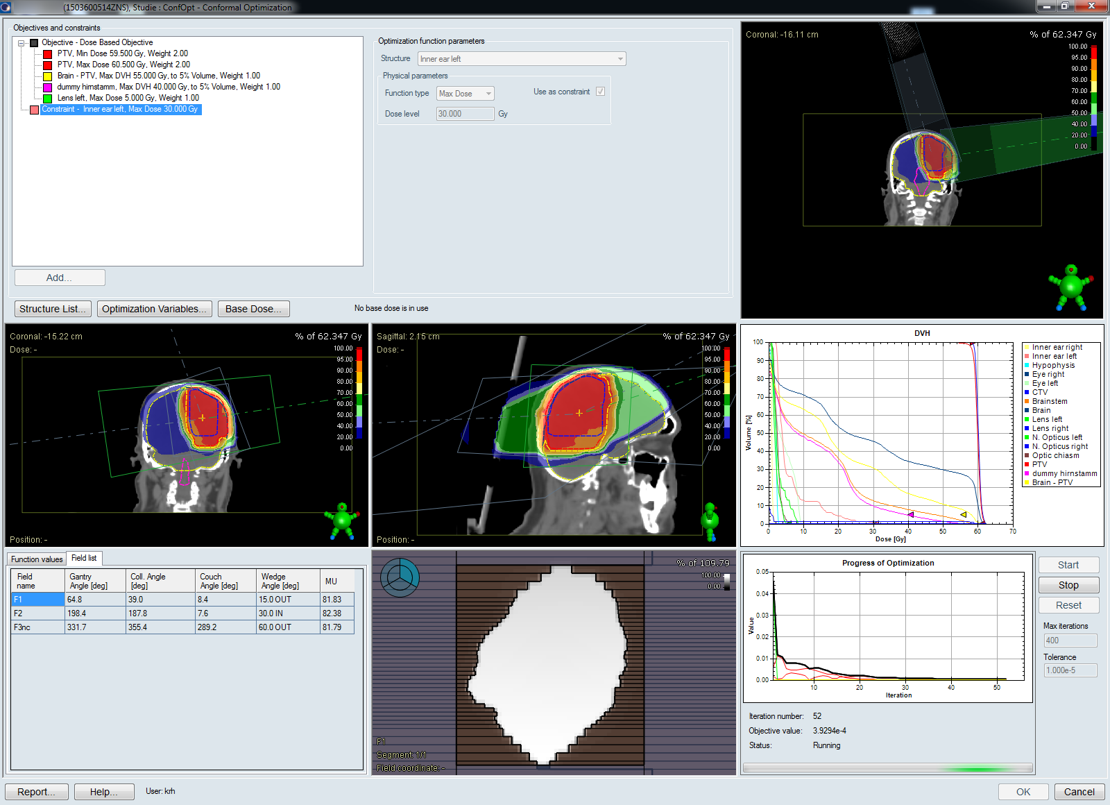
We define Objectives and Constraints for some OARs and repeat the optimization. Now it is significantly harder for the algorithm to find a good solution:
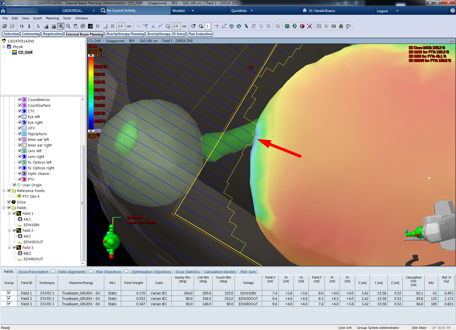
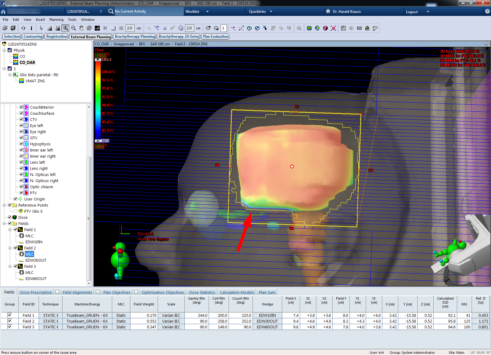
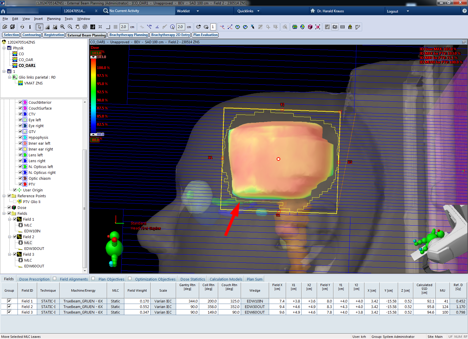
After 3D dose calculation, CO plans with OAR objectives usually have a low 3D Min for the PTV (46.1% in this case). This is because CO uses the static MLC to shield OARs, but this can locally reduce PTV dose (BEV of Field 3, shielding of N. opticus left). In such a case, since it is often a local effect, it is worth navigating to the location of the target dose minimum and to check in Beam's Eye View whether a manual "fine-tuning" of some MLC leaf position (here at the caudal edge of the PTV) could restore PTV dose a little, without significantly increasing OAR dose:
CO cannot "know" about such local interrelations, because it is only responding to DVH requirements and dose limits, which are valid for the whole structure.
After modifying a few leaves, the target dose minimum in this case improved from 46.1% to 71.1%:
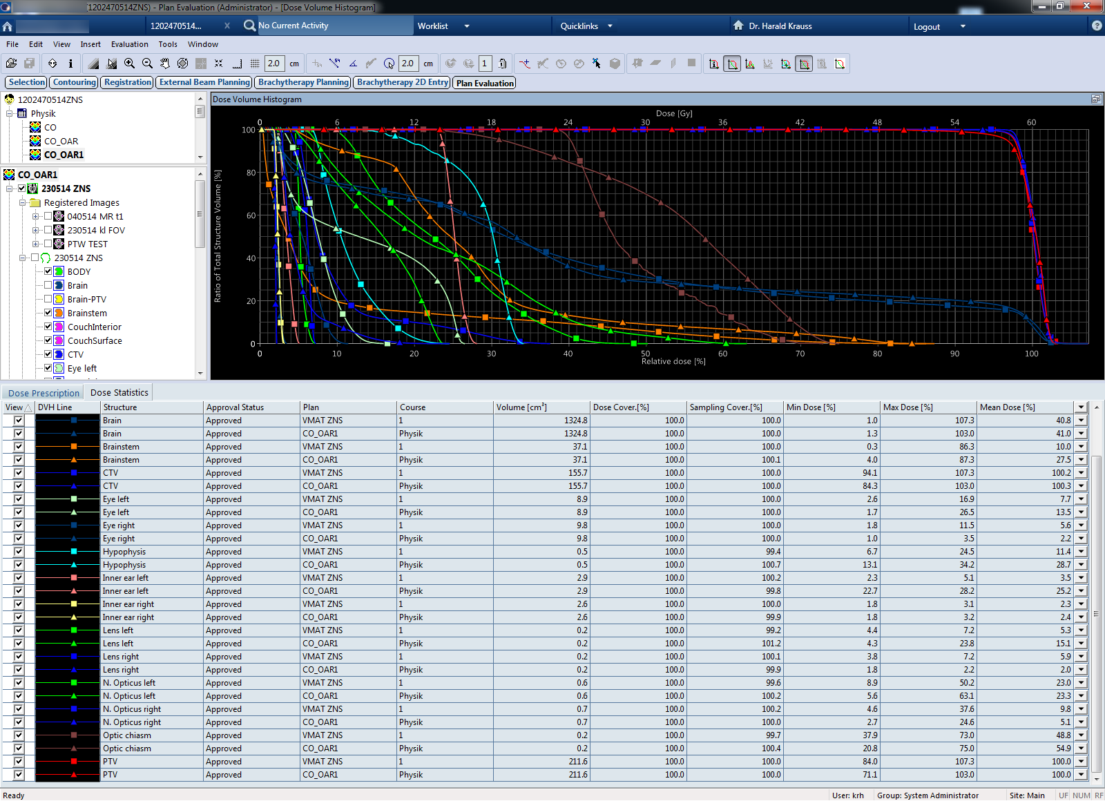
Of course, the impact of such a "fine-tuning" on the OAR's dose distributions and DVHs has to be observed. Here is the comparison of the CO plan and the clinical VMAT plan. OARs are now much better, and the CO plan is less than miles away from the VMAT plan:
This example showed the process of creating an optimized conformal plan with CO. Plan quality was better than for a manually set up plan (without proof), but still could not reach the quality of the VMAT plan4.
Discussion and Conclusion
CO works best (i.e., converges fast), if a target is not too close to important OARs. In such a case, it is sufficient to define objectives for the PTV alone, and CO will typically find a solution quickly that is better than the manual plan.
If OARs have to be included in the optimization, the type of function (Min/Max Dose, Min/Max DVH, Objective or Constraint) and the Weight of the function are important. This is where user experience helps. If, for instance, OAR objectives are too tight, the optimization will not converge and the solution will be suboptimal. Constraints should be used with caution, because they are really meant as "hard constraints", with no weight.
In the above example, all weights were set to 1 for simplicity. After some OARs had been included in the optimization, plan quality improved and actually came quite close to the clinically delivered VMAT plan (well, at least at first sight). However, the limits of the method are clear due to the principle: because in-field modulation is not possible, plan quality will never reach the quality of IMRT or VMAT plans.
One should also take into account that for getting a good CO plan, nearly the same time has to be spent as for the optimization of an IMRT or VMAT plan, since the basic steps are the same: Objectives have to be defined, the optimization loop takes time, and finally 3D dose is calculated.
Therefore, CO is probably only attractive for departments where neither IMRT nor VMAT are available.
Notes
1This does not mean that we consider wedged fields as IMRT. Not even if the wedges are dynamic.
2When seeing this for the first time, the user usually thinks that Eclipse has just crashed.
3While in the loop, the angle deltas between optimization steps are quite small.
4Since the example was only created for the website, it was not reviewed and optimized to the full extent. It should only demonstrate how CO works in principle.